Tutorial: Flow Cytometry Analysis with densitree#

This tutorial walks through a complete SPADE analysis of CyTOF data using the Levine_32dim benchmark dataset.

Setup#

import numpy as np
import pandas as pd
import matplotlib
matplotlib.use("Agg")  # use interactive backend if in a notebook
import matplotlib.pyplot as plt
from densitree import SPADE

Load data#

densitree works with numpy arrays or pandas DataFrames. Here we load the Levine_32dim benchmark dataset:

# If you have readfcs installed:
import readfcs
adata = readfcs.read("Levine_32dim.fcs")
df = adata.to_df()

# Select marker columns (exclude metadata like Time, DNA, etc.)
markers = [c for c in df.columns if c.startswith("CD") or c == "HLA-DR" or c == "Flt3"]
X = df[markers]
print(f"Data: {X.shape[0]} cells, {X.shape[1]} markers")

Run SPADE#

For CyTOF data, use arcsinh transform with cofactor 5:

spade = SPADE(
    n_clusters=50,           # overcluster for tree exploration
    downsample_target=0.1,   # retain 10% of cells
    knn=10,                  # k for density estimation
    transform="arcsinh",
    cofactor=5.0,            # CyTOF standard
    random_state=42,
)
spade.fit(X)

print(f"Clusters: {len(np.unique(spade.labels_))}")
print(f"Tree nodes: {spade.result_.tree_.number_of_nodes()}")
print(f"Tree edges: {spade.result_.tree_.number_of_edges()}")

Explore results#

Cluster statistics#

stats = spade.result_.cluster_stats_
print(stats.head(10))

# Find the largest and smallest clusters
print("\nLargest clusters:")
print(stats.nlargest(5, "size")[["size"]])

print("\nSmallest clusters (potential rare populations):")
print(stats.nsmallest(5, "size")[["size"]])

Visualize the tree#

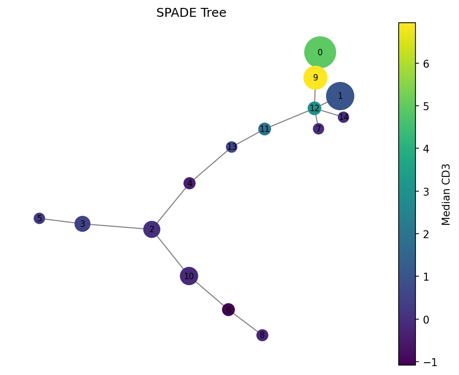
# Color by CD3 expression
fig = spade.result_.plot_tree(color_by="CD3", size_by="count", backend="matplotlib")
fig.savefig("spade_tree_cd3.png", dpi=150, bbox_inches="tight")

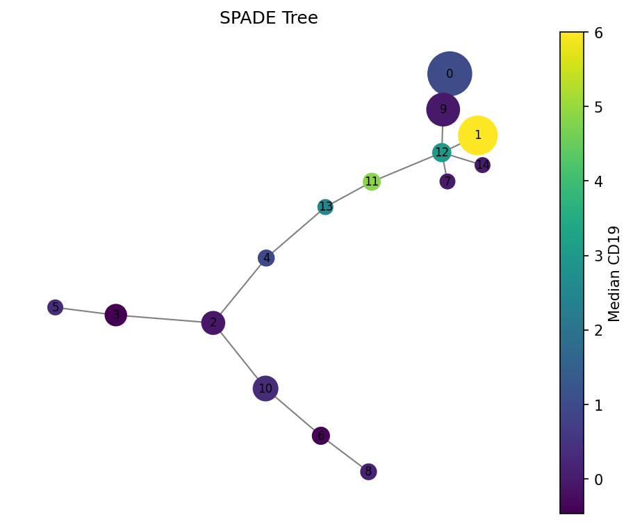
# Color by CD19 (B cell marker)
fig = spade.result_.plot_tree(color_by="CD19", size_by="count", backend="matplotlib")
fig.savefig("spade_tree_cd19.png", dpi=150, bbox_inches="tight")

Interactive exploration with plotly#

fig = spade.result_.plot_tree(color_by="CD3", backend="plotly")
fig.write_html("spade_tree_interactive.html")
# or fig.show() in a notebook

Work with the tree directly#

import networkx as nx

tree = spade.result_.tree_

# Find hub clusters (high degree = many connections)
degrees = sorted(tree.degree, key=lambda x: x[1], reverse=True)
print("Hub clusters:", degrees[:5])

# Find clusters connected to a specific node
neighbors = list(tree.neighbors(0))
print(f"Cluster 0 is connected to: {neighbors}")

# Get the path between two clusters (differentiation trajectory?)
path = nx.shortest_path(tree, source=0, target=25, weight="weight")
print(f"Path: {path}")
print("Markers along path:")
for node in path:
    median = tree.nodes[node]["median"]
    print(f"  Cluster {node}: size={tree.nodes[node]['size']}")

Export results#

# Add cluster labels to original data
df_out = X.copy()
df_out["spade_cluster"] = spade.labels_
df_out.to_csv("annotated_cells.csv", index=False)

# Export cluster statistics
spade.result_.cluster_stats_.to_csv("cluster_stats.csv")

# Export tree for external tools
nx.write_graphml(spade.result_.tree_, "spade_tree.graphml")

Parameter tuning tips#

If you see…	Try…
Too many small clusters	Decrease `n_clusters`
Rare populations missing	Increase `downsample_target` (e.g., 0.2) or decrease `knn`
Noisy tree with many short edges	Increase `n_clusters` to spread out populations
Very slow	Decrease `downsample_target` (e.g., 0.05)
For fluorescence flow cytometry	Use `cofactor=150.0` instead of 5.0